Dynamic routing protocols are used by Layer 3 network devices to automatically share routing information. Various routing protocols have been developed over the years, but most fall into one of three categories:
- Interior Gateway Protocol – Distance vector, such as EIGRP or RIP
- Interior Gateway Protocol – Link state, such as OSPF or IS-IS
- Exterior gateway protocol – Path vector, such as BGP
In this article, we’ll be comparing the characteristics of the two types of Interior Gateway Protocols (IGPs), specifically we’ll discuss Link State vs Distance Vector dynamic routing protocols.
Distance Vector Routing Protocols
Distance vector routing protocols are characterized by the fact that they determine the best path to a particular destination based on the distance to that destination.
Distance is measured in several ways. For example, RIP uses a hop count as the distance, simply the number of routers you must traverse to get to the destination.
Other distance vector protocols such as EIGRP use additional parameters to perform more efficient routing.
For example, EIGRP can be configured to take into account network latency, link bandwidth, as well as traffic load, and reliability when making routing decisions.
Routers participating in a distance vector routing protocol periodically exchange routing information with neighboring routers.
Typically, it is the routing table itself as well as hop counts and other network traffic-related information that is shared among routers.
Routers rely solely on the information from neighboring routers and do not assess the whole network topology when making routing decisions.
The name “distance vector” comes from the fact that such a protocol uses vectors (also called arrays in mathematical language or direction of the route) and distances to other nodes on the network.
It analyzes those distances to determine the best path. Distance vector routing protocols use the Bellman-Ford algorithm to calculate the best route.
Routers using distance vector routing protocols do not maintain information about the whole network topology, but only of the routers to which they are directly connected.
Each router advertises the distance to the networks it has learned about and receives information about networks its neighbors have learned about.
This process continues until the routing tables of all the participating routers have stabilized. This is called convergence.
Examples of distance vector routing protocols include:
Routing Information Protocol (RIP) – uses only hop count as the measure of distance
Interior Gateway Routing Protocol (IGRP) – uses multiple metrics for each route including bandwidth, delay, load, and reliability. It is currently considered obsolete and should not be implemented in production networks.
Enhanced Interior Gateway Routing Protocol (EIGRP) – often called an “advanced distance vector routing protocol,” which sends only incremental updates which reduces the workload on the router and the amount of data to be transmitted.
Basic Example of Distance Vector Topology
The following topology shows a basic example of a simple Distance Vector routing algorithm (such as RIP for example):
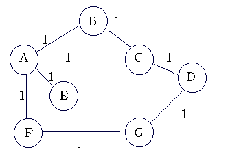
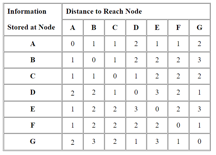
Each Node above represents a router device in a network. After the above network topology is stabilized (converged), here are the final distances stored at each Node in the network:
Link State Routing Protocols
Link state routing protocols are characterized by the fact that every node maintains a complete map of the network topology in the form of a graph, or a database.
Within this database, each individual router knows which routers are connected to which other routers.
Based on this complete map of the network, each router will independently calculate the best path to every possible destination in the network. This calculated best path is then installed within the routing table.
The information shared between link state routers is connectivity related and is contained within what is known as a link state advertisement (LSA).
These LSAs are shared in such a way that each participating router will have received an LSA from every node on the network.
With the complete set of LSAs, a router produces a network map. The routing protocol is said to have converged when all routers in the topology have constructed the same network topology within their databases.
This network map is then analyzed and a shortest path tree is created. This is a data structure that simply determines the best path to each destination based on the network topology and the link cost information that has been shared via the LSAs. From this tree, the routing table is then constructed.
Examples of link state routing protocols include:
Open Shortest Path First (OSPF) – among the most popular IGPs in production networks today
Intermediate System to Intermediate System (ISIS) – most often used by ISPs for their internal networks
Basic Example of Link State Topology
The following topology shows a basic example of a simple Link State network topology.
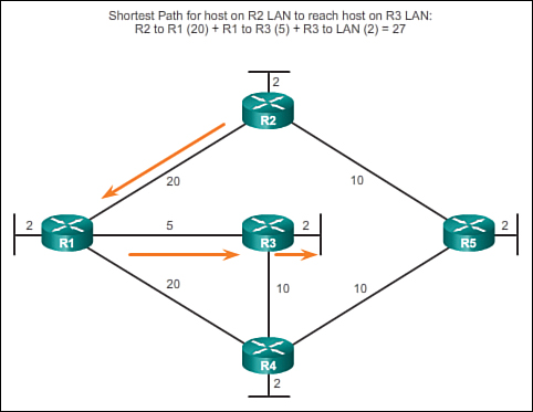
This algorithm uses accumulated costs along each path, from source to destination, to determine the total cost of a route. The cost of each path is determined by the routers using various factors such as speed of the link etc.
Comparison of Distance Vector vs Link State Protocols
EIGRP and OSPF are often considered flagship protocols of each type. Both are highly functional, and scalable, and have been extensively deployed worldwide.
The most striking differences between them help to highlight the differences between distance vector and link state routing protocols. These differences include:
- EIGRP has a flat structure and is highly scalable, while OSPF has a hierarchical structure to accommodate larger networks. This hierarchical structure results in an OSPF topology being separated into distinct areas.
- EIGRP’s metric or distance is determined using a complex formula that takes various parameters into account while OSPF determines the metric based on the cumulative cost along the path to a particular destination.
Comparison Table of Distance Vector and Link State
The following table contains a more detailed look at the differences between these two routing protocol types.
| Distance Vector | Link State | |
| Algorithm | Bellman-Ford | Dijkstra’s algorithm |
| Algorithm characteristics | Slower but more versatile | Faster but less versatile |
| Routers share | Routing tables | Link State Advertisements |
| Network | Knows only information from directly connected routers | Maintains a complete map of the network topology |
| Best path calculated | Based on shortest distance | Based on cost (link state) |
| Resource usage | Low | High |
| Convergence time | Fast | Very fast |
| Structure | Flat | Hierarchical |
| Border nodes | No | Yes |
| Complexity of deployment | Relatively simple | Somewhat more involved |
| Examples | RIP, IGRP, EIGRP | OSPF, ISIS |
Conclusion
Both link state and distance vector routing protocols have been around for almost half a century, so the technology in which these are based is extremely mature.
Each type delivers more than sufficient dynamic routing capabilities for most implementations. However, knowing the differences between them can help you make the decision of which to use in your situation.
Related Posts
- Difference Between Routers and Switches in TCP/IP Networks
- 11 Different Types of IP Addresses Used in Computer Networks
- Compare and Contrast Network Topologies (Star, Mesh, Bus, Hybrid etc)
- 11 Networking Companies Like Cisco (Competitors)
- What is a Wildcard Mask – All About Wildcard Masks Used in Networking