Classful and Classless addressing are two methodologies used in the allocation and identification of IP addresses within the Internet Protocol Version 4 (IPv4) framework.
Classful addressing, which was the initial scheme, divides the IP address space into classes which determines each network’s size and its division between network and host identifiers.
In contrast, classless addressing allows for a more flexible allocation of IP addresses by using a variable-length subnet mask (VLSM) to specify the division between the network portion and the host portion of an address, thus optimizing the utilization of the available address space.
In this article, we’ll examine these two approaches explaining their differences, limitations, and use cases.
Classful Design of IPv4
When IPv4 was designed in the very early 1980s, most host devices were very simple terminals with limited capabilities.
IP Network addressing was supposed to be a very simple process of just issuing the 32-bit IP address. No fields for subnet mask and other network parameters were even conceived.
For this reason, the designers of IPv4 decided to include in the design a hardwired subnet mask. This hardwired mask simply stated that IP addresses in a particular range will always get the same subnet mask.
Said differently, IP addresses in a particular class will always get the same subnet mask. So, in this sense, IPv4 was initially created to have a classful approach to IPv4 addressing.
IPv4 Classes
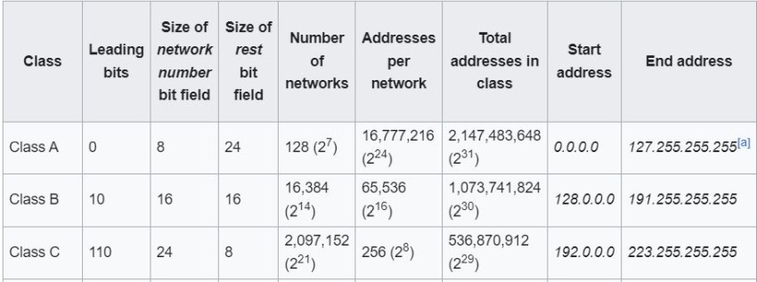
So IPv4 addresses were separated into five classes. These classes were defined based on the leading bits or leftmost bits of the IP address. By definition, the leading bits of each class are as follows:
|
CLASS |
Leading Bits |
|
Class A |
0 |
|
Class B |
10 |
|
Class C |
110 |
|
Class D |
1110 |
|
Class E |
1111 |
Now classes A, B, and C are the classes that are used for general IP addressing. Class D is reserved for IPv4 multicast addresses and Class E was initially reserved for future use, experimental use, and for research, and as of yet they are still not used for general networking purposes.
As far as classful IP addressing schemes go, we use classes A, B, and C, and it is these classes that we will examine in this article.
Class A addresses
To further understand how these addresses are classified, let’s take a look at the whole of the class A IPv4 address space in binary. A class A IP address in binary looks like this:
0XXXXXXX.XXXXXXXX.XXXXXXXX.XXXXXXXX
Where the leading bit is 0, and the rest of the bits can be either 0 or 1. So the address range of class A addresses in binary can be seen here:
00000000.00000000.00000000.00000000
…
01111111.11111111.11111111.11111111
Now translating that to the more familiar dotted decimal format, we get a range of:
0.0.0.0 to 127.255.255.255
Class B addresses
We can perform a similar exercise for class B addresses. Remember, class B addresses have leading bits of 10 in binary:
10XXXXXX.XXXXXXXX.XXXXXXXX.XXXXXXXX
So the address range of class B addresses in binary can be seen here:
10000000.00000000.00000000.00000000
…
10111111.11111111.11111111.11111111
Now translating that to the more familiar dotted decimal format, we get a range of:
128.0.0.0 to 191.255.255.255
Class C addresses
We can do the same thing for class C addresses. Remember, class C addresses have leading bits of 110 in binary:
110XXXXX.XXXXXXXX.XXXXXXXX.XXXXXXXX
So the address range of class B addresses in binary can be seen here:
11000000.00000000.00000000.00000000
…
11011111.11111111.11111111.11111111
Now translating that to the more familiar dotted decimal format, we get a range of:
192.0.0.0 to 223.255.255.255
IPv4 Classes and Subnet Masks
So to summarize, the three ranges of class A, B, and C IPv4 addresses are:
- Class A: 0.0.0.0 to 127.255.255.255
- Class B: 128.0.0.0 to 191.255.255.255
- Class C: 192.0.0.0 to 223.255.255.255
Now that we know how these are derived, let’s take a look at how they are used practically. The advantage of a classful address is that when you configure it on a device, you simply configure the address. No subnet mask needs to be configured.
In fact, you don’t have to configure anything else! This may seem like a small benefit, but at the time, when even the least bit of innovation in computing was costly, reducing even the number of fields you need to fill out to configure the network parameters of a device was of benefit.
So addresses of each class had a predefined subnet mask. If you configured a device to be in a Class B address range, for example, the subnet mask was automatically configured for you internally to the device. It was part of the protocol.
So, what are those predetermined subnet masks? Well, here they are:
- Class A mask: 255.0.0.0
- Class B mask: 255.255.0.0
- Class C mask: 255.255.255.0
Why were these chosen? Well, it was really a matter of convenience. The dotted decimal format had dots between octets, so why not just set the subnet masks to match up with those dots?
Devices couldn’t care less what subnet mask would be used. But for humans, this way they can be written out much more easily.
Inefficiencies of Classful Addressing
In classful addressing, the IP address space is divided into specific classes with fixed-sized network and host portions, based on these predefined subnet masks. This led to many wasted addresses in some classes and a shortage in others.
For example, the network 12.0.0.0 which uses a class A subnet mask of 255.0.0.0 allows for over 16 million host addresses.
However, practically speaking, IP subnet sizes never surpass several hundred hosts due to problems with broadcasts. So millions of IP addresses are wasted. At the same time, only 126 class A subnets are available, excluding the reserved 0.0.0.0 and 127.0.0.0 subnets. These range from:
- 1.0.0.0
- 2.0.0.0
- 3.0.0.0
- …
- 124.0.0.0
- 125.0.0.0
- 126.0.0.0
As you can imagine, simply looking at the class A address space as described above, we have tens of millions of wasted IPv4 addresses distributed among 126 networks.
Similar scalability problems exist with class B and class C addresses as well.
As time went on, and the infant Internet began to grow, this approach very quickly proved to be too restrictive and wasteful.
So, by 1993, classless addressing was introduced. This simply meant that the classes that had been originally defined were essentially abolished.
Classless IPv4 Addressing
Classless IP addressing essentially allows you to choose any subnet mask you like for your IP addresses without needing to adhere to the classful restrictions.
So, you can create a network with a network address of 10.20.55.0, for example, and use a subnet mask of 255.255.255.128 to provide a subnet with a range of IP addresses from 10.20.55.0 – 10.20.55.127.
You can do this even though this is a class A address and would otherwise require a 255.0.0.0 subnet mask.
Similarly, you could have an address of 193.75.0.0 and use a subnet mask of 255.255.0.0, even though this is a Class C address and would otherwise require a 255.255.255.0 subnet mask.
Related Concepts
With the advent of classless IPv4 addressing, there are a couple of related concepts that I’m sure you’ve heard about if you’re involved with networking. The first of these is Variable Length Subnet Masking or VLSM.
VLSM
While classful addressing had three possible subnet masks, classless not only allows you to mix and match these masks, but it allows you to have subnet masks of any length.
This is called Variable Length Subnet Masking, allowing you to create subnets of multiple sizes. Here for example you can see several different subnet mask sizes. In this list, we write out the last two octets in binary to more clearly show the variable length of the subnet mask, and we have made the host bits bold:
- 255.255.11111100.00000000 255.255.252.0
- 255.255.11111110.00000000 255.255.254.0
- 255.255.11111111.00000000 255.255.255.0
- 255.255.11111111.10000000 255.255.255.128
- 255.255.11111111.11000000 255.255.255.192
- 255.255.11111111.11100000 255.255.255.224
- 255.255.11111111.11110000 255.255.255.240
- 255.255.11111111.11111000 255.255.255.248
By using VLSM, you have the freedom to create subnets that are closer in size to the actual number of hosts that you are expected to have within a subnet.
CIDR
The second related concept is called Classless Interdomain Routing or CIDR. Similarly, CIDR is a function that allows a router to route these “classless” networks, taking into account additional subnet information to decide how to route packets.
This is in contrast to routing based on classful IP address network boundaries. Classless IP addressing is sometimes referred to as CIDR, although it’s not quite the same thing. The former has to do with address allocation, while the latter has to do with routing those classless addresses.
Best Practices
It should be made perfectly clear that in modern networks that use IPv4 addressing, only classless addressing should be implemented.
All current equipment supports classless addressing, so unless you are using equipment that is close to two decades old, you should ensure that classless addressing is employed.
Even so, it is important to understand classful IPv4 addressing because it is an inherent part of the development of IPv4. To fully understand and appreciate classless addressing, an understanding of the classful approach is necessary.
Keep in mind that even in the most cutting-edge network device, you will still see evidence of the classful nature of IPv4.
In some commands in Cisco routers, if you omit the subnet mask or wildcard mask, they will assume a classful address. Similarly, the routing table of a Cisco router will group routes in a classful manner when it displays them.
Conclusion
The transition from classful to classless IPv4 addressing has significantly improved the efficiency and scalability of IP address allocation, mitigating the rapid exhaustion of available addresses in the face of the Internet’s explosive growth.
By adopting classless addressing and the related concepts of VLSM and CIDR, a more efficient use of the limited IP4 space can be achieved, paving the way for more sustainable IPv4 network management.
Related Posts
- Difference Between Routers and Switches in TCP/IP Networks
- 11 Different Types of IP Addresses Used in Computer Networks
- Compare and Contrast Network Topologies (Star, Mesh, Bus, Hybrid etc)
- 11 Networking Companies Like Cisco (Competitors)
- What is a Wildcard Mask – All About Wildcard Masks Used in Networking